• Calculus > Cycloidal Curves

The Cycloidal Curves

Circles Rolling on Top of Curves

Suppose a circle with radius r rolls along a curve f(x), and the circle starts at a point where f crosses the y-axis. A point on the circle traces a curve given by parametric equations C(x, y). What are the equations that define this path for the curve C? We know that when f(x) = 0, the curve is the cycloid. But we want to extend this to all curves f(x).

We will find the path of the curve for a circle that “rolls on top” of the curve. First, we must find the curve P(x, y) that is traced by the center of the circle. This curve is parallel to f. A tangent line has been drawn at point (x_t, f(x_t)). The angle φ will enable us to find the curve P. The angle created by the tangent and the x-axis is equal to φ. Therefore, the measure of φ is given by:

(i) \(\phi = \arctan(f'(x_t))\)

From (i), we can determine the position of point P. First, note that when the tangent has a slope of 0, then x_p = x_t. When slope of the tangent is negative (as depicted in the picture), then φ is negative; therefore, \(x_p = x_t - r\sin\phi\). When the slope of the tangent is positive, then φ is positive; therefore, \(x_p = x_t - r\sin\phi\) still holds true. Thus, the point x_p is given by: \(x_p = x_t - r\sin\phi =\) \(x_t - r\sin[\arctan(f'(x_t))] =\) \(x_t - \frac{r\cdot f'(x_t)}{\sqrt{1+[f'(x_t)]^2}}\).

(ii) \(x_p = x_t - \frac{r\cdot f'(x_t)}{\sqrt{1+[f'(x_t)]^2}}\)

Now, finding y_p is similar to finding x_p. Without difficulty, y_p can be determined to be:

(iii) \(y_p = f(x_t) + r\cos\left[\arctan(f'(x))\right] = f(x_t) + \frac{r}{\sqrt{1+[f'(x_t)]^2}}\)

Therefore, P is given by the parametric equations: \(x_p = x_t - \frac{r\cdot f'(x_t)}{\sqrt{1+[f'(x_t)]^2}}\) and \(y_p = f(x_t) + \frac{r}{\sqrt{1+[f'(x_t)]^2}}\).

Now, we turn to finding the angles θ₀ and θ₁. The angle θ₀ is the initial θ angle created by the circle when x_t = 0. The exact measure of θ₀ need not be determined because it will cross out later. The measure of angle θ₁ (which is angle F₁PO that overlaps with angle φ) is given by:

(iv) \(\theta_1 = \frac{\pi}{2} + \phi - \theta_0\)

Measure of angle θ₂ can be found by noticing that the length of the arc, FC, of the circle (going clockwise) is equal to the arc length of the curve f from x = 0 to x = x_t. In other words: \(r\theta_2 = \int_{0}^{x_t}\sqrt{1+[f'(x)]^2}\text{ }dx\). Therefore, we have the relationship:

(iv) \(\theta_2 = \frac{1}{r}\int_{0}^{x_t}\sqrt{1+[f'(x)]^2}\text{ }dx\)

From the figure, we can also see that θ + θ₀ + θ₁ + θ₂ = 2π. This gives us the relationship for θ: θ = 2π – θ₀ – θ₁ – θ₂. Let’s substitute θ₁ that we got in (iv): \(\theta = 2\pi - \theta_0 - (\frac{\pi}{2} + \phi - \theta_0) - \theta_2 = \) \(\frac{3\pi}{2} - \phi - \theta_2\). This gives us the θ that we need.

(v) \(\theta = \frac{3\pi}{2} - \arctan(f'(x)) - \) \(\frac{1}{r}\int_{0}^{x_t}\sqrt{1+[f'(x)]^2}\text{ }dx\)

Knowing θ, we can find the coordinates C(x_c, y_c). We can easily relate the following: \(x_c = x_p + r\cos\theta\) and \(y_c = y_p + r\sin\theta\). Using the sum identity of sine and cosine, we can simplify cos(θ) and sin(θ) to remove the 3π/2 as: \(\cos\theta = \sin\left[ \arctan(f'(x_t)) - \frac{1}{r}\int_{0}^{x_t}\sqrt{1+[f'(x)]^2}\text{ }dx \right]\) and \(\sin\theta = -\cos\left[ \arctan(f'(x_t)) - \frac{1}{r}\int_{0}^{x_t}\sqrt{1+[f'(x)]^2}\text{ }dx \right]\).

(Note that we changed the variable x_t to simply t.)

Finding the equations of the curve depends highly on being able to evaluate the integral for the arc length. Many curves give integrals that can be evaluated. Some curves, like the sine curve, do not result in a nice integral. I was able to graph the function, however, with the integral using Desmos. This curve is shown below.

The Cycloid

We already know that when f(x) = 0, the curve should reduce to a cycloid. We will demonstrate that this does, in fact, occur:

\(x(t) = t - \frac{r\cdot 0}{1+[0]^2} + \) \( r\sin\left[ \arctan(0) - \frac{1}{r}\int_{0}^{t}\sqrt{1+[0]^2}\text{ }dx \right] = \) \(t-r\sin\frac{t}{r}\), and

\(y(t) = 0 + \frac{r}{1+[0]^2} - \) \(r\cos\left[ \arctan(0) - \frac{1}{r}\int_{0}^{t}\sqrt{1+[0]^2}\text{ }dx \right] = \) \(r - r\cos\frac{t}{r}\).

Note that x_t = rθ₁ or t = rθ₁. Therefore, these equations can be written as: \(x(r\theta_1) = r\theta_1 - r\sin\theta_1\) and \(y(r\theta_1) = r - r\sin\theta_1\). Since r is a scalar and rθ₁ will take on all values we allow, we can treat rθ₁ as just θ. Thus, these equations simplify to the equations of the cycloid: \(x(\theta) = r\theta - r\sin\theta\) and \(y(\theta) = r - r\sin\theta\). However, to show that the above equations are that of a cycloid, the parametric equation without manipulation is graphed below. The cicle has a radius of 2 in the image below.

Other Curves

Slanted Cycloid

When f(x) = x, a line with slope of 1, we have the equations:

\(x(t) = t - \frac{r}{\sqrt{2}} + r\sin\left(\frac{\pi}{4}-\frac{\sqrt{2}}{r}t\right)\) and

\(y(t) = t + \frac{r}{\sqrt{2}} - r\cos\left(\frac{\pi}{4}-\frac{\sqrt{2}}{r}t\right)\).

This is the cycloid generated on the line y = x. The graph for this curve is shown below (for r = 1).

Rolling on a Parabola

Actually, let’s roll on a horizontal parabola first. When \(f(x) = \sqrt{x}\), then:

\(x(t) = t-\frac{r}{\sqrt{4t+1}} + \) \( r\sin\left[ \arctan\frac{1}{2\sqrt{t}} - \frac{1}{4r}\sinh^{-1}(2\sqrt{t})-\frac{1}{2r}\sqrt{t+4t^2} \right]\) and

\(y(t) = \sqrt{t}+\frac{r}{\sqrt{1+\frac{1}{4t}}} - \) \( r\cos\left[ \arctan\frac{1}{2\sqrt{t}} - \frac{1}{4r}\sinh^{-1}(2\sqrt{t})-\frac{1}{2r}\sqrt{t+4t^2} \right]\).

The graph is shown below (for r = 1):

When f(x) = x², we have:

\(x(t) = t - \frac{2rt}{\sqrt{1+4t^2}} + \) \( r\sin\left[ \arctan(2t) - \frac{1}{4r}\sinh^{-1}(2t)-\frac{t}{2r}\sqrt{1+4t^2} \right]\) and

\(y(t) = t^2 + \frac{r}{\sqrt{1+4t^2}} - \) \( r\cos\left[ \arctan(2t) - \frac{1}{4r}\sinh^{-1}(2t)-\frac{t}{2r}\sqrt{1+4t^2} \right]\).

The graph is shown below (for r = 1).

Trigonometric Functions

The curve below was generated for f(x) = sin(x).

\(x(t) = t-\frac{r\cos t}{\sqrt{1+\cos^{2}t}}+ \) \(r\sin\left[ \arctan(\cos t) - \frac{1}{r}\int_{0}^{t}\sqrt{1+\cos^{2}x}\text{ }dx \right]\)

\(y(t) = \sin t+\frac{r}{\sqrt{1+\cos^{2}t}}- \) \(r\cos\left[ \arctan(\cos t) - \frac{1}{r}\int_{0}^{t}\sqrt{1+\cos^{2}x}\text{ }dx \right]\)

Because the integral has no closed form, we have left the integral as is. The image is below:

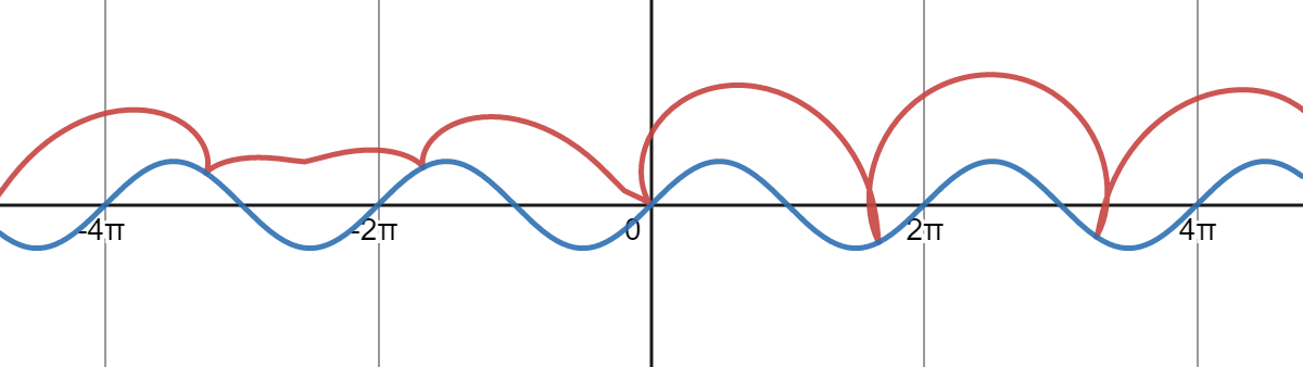
Because of the curvature of the sine curve around 3π/2, there a small loop created.

If we let r ≈ 0.608, then the circumference of the circle is about C ≈ 3.8202. The circumference of this circle is approximately equal to the arc length of the sine curve from 0 to π. The following graph shows the curve that corresponds to this situation:

The cusps match quite nicely at the x-intercepts of the sine curve.

Exponential/Logarithmic Curves

When \(f(x) = \ln(x)\), then the cycloidal curve is given by:

\(x(t) = t - \frac{r}{\sqrt{1+t^2}} + \) \( r\sin\left[ \arctan\frac{1}{t} - \frac{1}{r}\sqrt{1+t^2} + \frac{1}{r}\sinh^{-1}\frac{1}{t} \right]\) and

\(y(t) = \ln t + \frac{rt}{\sqrt{1+t^2}} - \) \(r\cos\left[ \arctan\frac{1}{t} - \frac{1}{r}\sqrt{1+t^2} + \frac{1}{r}\sinh^{-1}\frac{1}{t} \right]\)

The graph is shown below:

Circle rolling on \(f(x) = e^x\) curve:

\(x(t) = t - \frac{r\cdot e^t}{\sqrt{1+e^{2t}}} + \) \( r\sin\left[ \arctan(e^t) - \sqrt{e^{2t}+1} + \tanh^{-1}\sqrt{e^{2t}+1} \right]\) and

\(y(t) = e^t + \frac{r}{\sqrt{1+e^{2t}}} - \) \(r\sin\left[ \arctan(e^t) - \sqrt{e^{2t}+1} + \tanh^{-1}\sqrt{e^{2t}+1} \right]\) and

Circles Rolling on Bottom of Curves

The equations below give the cycloid created on the bottom (or outside) the parabola.

\(x(t) = t + \frac{2rt}{\sqrt{1+4t^2}} - \) \( r\sin\left[ \arctan(2t) - \frac{1}{4r}\sinh^{-1}(2t)-\frac{t}{2r}\sqrt{1+4t^2} \right]\) and

\(y(t) = t^2 - \frac{r}{\sqrt{1+4t^2}} + \) \( r\cos\left[ \arctan(2t) - \frac{1}{4r}\sinh^{-1}(2t)-\frac{t}{2r}\sqrt{1+4t^2} \right]\).

Note that only the signs changed in the formulas for circles rolling over or on the bottom. This is the same effect we get when the radius is negative.

Anirdesh.com