• Calculus > Tangent-generated Curve

The Tangent-generated Curve

In around March of 1999, I started investigating a special curve that arose from its tangents. I embarked on finding the equation of this curve which was inspired from my elementary school art class.

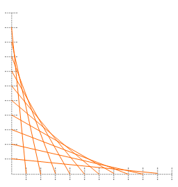
In our art class, we used string to generate some fancy designs on a wooden board with tacks placed incrementally. We drew two perpendicular segments and divided them into an x units. At each division, we nailed in a small tack. Then we took colored string and looped them around the tacks from one segment to the other sequentially as can be seen in the image. The vertical segment is numbered 1 to x from top to bottom. The horizontal segment is numbered 1 to x from left to right. Hence, you loop the string 1 to 1, 2 to 2, 3 to 3, and so on. Depending on the the angle and number of increments, you can come up with different designs.

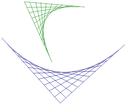
Well, years later, I recalled this artwork and started to wonder about the curve that is generated by all these lines. If you had time to draw infinite lines, you would produce a curve from all these lines. My persistence to characterize this curve paid off with a familiar equation that we’ll investigate here. I resorted to differential equations and my y-intercept and x-intercept formulas to find the equation of this curve. Knowing these lines are tangents will help us derive the equation.

I have not come up with a general equation for curves generating from segment angles other than 90°. I have come up with an equation for segments that are perpendicular and have different lengths, L₁ and L₂. The segments are on x-axis and y-axis.

Derivation of the Equation

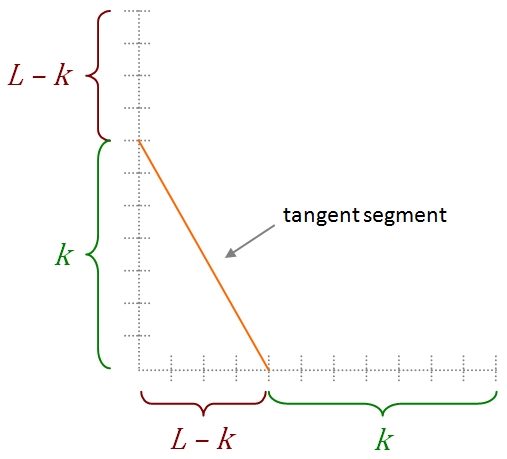
The simplest case is when both segments are equal in length. In this case, the tangent segment (which is a segment of the tangent line from the y-axis to the x-axis) can be considered as sliding against the y-axis. What ever distance it slides on the y-axis from the top is the distance it moves along the x-axis. Hence, the figure on the right shows the relationship with k being the distance the segment slides.

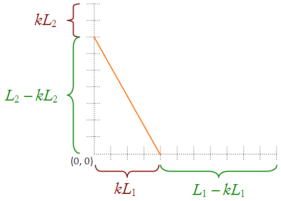
I will derive the equation for the segments being of unequal length, L₁ and L₂. At the end, we can let L₁ = L₂ = L to find the equation for equal lengths. I haven’t found an algebraic method, so I will resort to differential equations. Let’s begin.

In the figure on the left, L₂ is less than L₁. Hence, as it slides, the tangent segment gets bigger. The distance it slides on the x-axis is greater than the distance it slides down the y-axis. Hence, we introduce a factor, k, where 0 ≤ k ≤ 1, that will allows us to state the relationship between the way segments L₁ and L₂ are divided by the tangent segment.

Since we know where the tangent crosses the x-axis and y-axis, we have the following two relationships with the x-intercept and y-intercept formulas:

(i) \(y_{yi} = y-x\dfrac{dy}{dx}=L_2-kL_2\)

(ii) \(y_{xi} = x-y\dfrac{dx}{dy}=kL_1\)

Solving for k in one and substituting in the other gives:

(iii) \(y-x\dfrac{dy}{dx} = L_2 - L_2\left( \dfrac{x}{L_1}-\dfrac{y}{L_1}\cdot \dfrac{dx}{dy} \right)=\) \(L_2-\dfrac{L_2}{L_1}x + \dfrac{L_2}{L_1}y\dfrac{dx}{dy}\)

(iv) \(y\dfrac{dy}{dx} - x\left( \dfrac{dy}{dx} \right)^2 = L_2\dfrac{dy}{dx}-\dfrac{L_2}{L_1}x\dfrac{dy}{dx}+\dfrac{L_2}{L_1}y\) (Multiplying both sides of (iii) by dy/dx)

(v) \(y\dfrac{d^2 y}{dx^2} + \left( \dfrac{dy}{dx} \right)^2 - \left( \dfrac{dy}{dx} \right)^2 - 2x\cdot \dfrac{dy}{dx}\cdot\dfrac{d^2 y}{dx^2} = \) \(L_2\dfrac{d^2 y}{dx^2} - \dfrac{L_2}{L_1}\cdot\dfrac{dy}{dx}-\dfrac{L_2}{L_1}x\dfrac{d^2 y}{dx^2}+\dfrac{L_2}{L_1}\cdot \dfrac{dy}{dx}\) (Differentiating both sides)

(vi) \(y-2x\cdot\dfrac{dy}{dx}=L_2-\dfrac{L_2}{L_1}x\) (Simplifying (v) yields a surprisingly simple result)

Rearranging the equation reveals that it is a first-order linear differential equation:

(vii) \(\dfrac{dy}{dx}-\dfrac{1}{2x}y=\dfrac{L_2}{2L_1}-\dfrac{L_2}{2x}\)

The solution of (vii) is given by:

(viii) \( ye^{-0.5\int{(1/x)dx}}=\) \(\displaystyle\int \left( \dfrac{L_{2}}{2{L}_{1}}-\dfrac{L_{2}}{2x} \right)e^{-0.5\int{(1/x)}dx}dx+C\)

(ix) \(yx^{-0.5} = \) \(\displaystyle\int \left( \dfrac{L_2}{2L_1}-\dfrac{L_2}{2x} \right)x^{-0.5}\text{ }dx+C =\) \(\dfrac{L_2}{2} \displaystyle\int \dfrac{1}{L_1}x^{-0.5} - x^{-1.5}\text{ }dx+C\)

(x) \(yx^{-0.5} = \dfrac{L_2}{2}\left( \dfrac{2x^{0.5}}{L_1} + 2x^{-0.5} \right)+C\)

(xi) \(y=\dfrac{L_2}{L_1}x+L_2+C\sqrt{x}\)

One last step is to find C so that the equation fits our curve. When x = L₁, y = 0. Therefore: \(0=L_2+L_2+C\sqrt{L_1}\) and \(C=-\dfrac{2L_2}{\sqrt{L_1}}\).

Finally, we have our equation for the tangent-generated curve.

A curve generated by tangents that cross segments of length L₁ on the x-axis and L₂ on the y-axis is given by \(y=\dfrac{L_2}{L_1}x-2L_2\sqrt{\dfrac{x}{L_1}}+L_2\) or \(\sqrt{L_2x}+\sqrt{L_1y}=\sqrt{L_1L_2}\).

When L₁ = L₂ = L, the equation reduces to an elegant form.

A curve generated by tangents that cross segments of length L on the x-axis and the y-axis is given by \(y=x-2\sqrt{Lx}+L\) or \(\sqrt{x}+\sqrt{y}=\sqrt{L}\).

Graph and Symmetry

The image below shows the graph of the curve. Notice its symmetry with respect to line y = x (image not perfectly proportional). It’s quite easy to prove symmetry. We simply switch x and y and solve for y. For the equation, \(\sqrt{x}+\sqrt{y}=\sqrt{L}\), there’s no need to solve for y after the switch because we obtain the same thing.

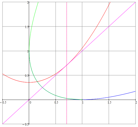
It’s interesting to note that, in the form \(\sqrt{x}+\sqrt{y}=\sqrt{L}\), the limits of x and y are 0 ≤ x ≤ L and 0 ≤ y ≤ L. So the graph of this equation is only the portion from 0 to L on the x- and y-axes. However, when we solve for y or x, we can extend the graph of this curve beyond L. The graph maintains its symmetry; but to see the full curve, we would have to solve for x and y and plot both equations. Both equations have been plotted in the image on the right shown as blue and green with L = 1. There’s overlap of green and blue, and this overlap represents the curve \(\sqrt{x}+\sqrt{y}=\sqrt{L}\). The curve can be rotated 45°. Turn it 45° and what do you see? Looks like a ... parabola? In the image, the x-axis is shown in magenta after rotation of 45° as a tangent line of the parabola in red with equation y = x.

The implicit derivative of the curve is \(\dfrac{dy}{dx} = -\sqrt {\dfrac{y}{x}}\). The y-intercept is given by \(y_{yi} = y + \sqrt{xy}\) and x-intercept is given by \(y_{xi} = x + \sqrt{xy}\).

Rotating the Curve

Let’s rotate the curve. A point in the xy-coordinate system rotated 45° clockwise is given by x' = xcosθ + ysinθ and y' = ycosθ - xsinθ. If you consider the curve is already in the x'y'-coordinate system, then we simply rotate it back 45°.

(i) \(\sqrt{x'}+\sqrt{y'}=\sqrt{L}\)

(ii) \(\sqrt{x\cos \dfrac{\pi}{4} + y\sin \dfrac{\pi}{4}}+\) \(\sqrt{y\cos \dfrac{\pi}{4}-x\sin \dfrac{\pi}{4}} = \sqrt{L}\)

(iii) \(\dfrac{\sqrt{2}}{2}(x+y)=\) \(L-2\sqrt{\dfrac{\sqrt{2}}{2}L(y-x)}+\) \(\dfrac{\sqrt{2}}{2}(y-x)\) (squaring both sides)

(iv) \(2\sqrt{\dfrac{\sqrt{2}}{2}L(y-x)}=L-\sqrt{2}x\) (rearranging and simplifying)

(v) \(4\cdot \dfrac{\sqrt{2}}{2}L(y-x) = L^2-2\sqrt{2}Lx+2x^2\) (squaring both sides again)

(vi) \(y=\dfrac{\sqrt{2}L}{4}+\dfrac{\sqrt{2}}{2L}x^2\)

This is indeed the equation of a parabola. So the curve is a parabola rotated by 45° clockwise. The parabola is shown in red in the image.

The equation of the tangent-generated curve is a parabola that has been rotated by 45° clockwise. The equation of the parabola before rotation is \(y=\dfrac{\sqrt{2}L}{4}+\dfrac{\sqrt{2}}{2L}x^2\).

The point \(\left( \dfrac{L}{4},\dfrac{L}{4} \right)\) is the closest point on the curve to the origin. The distance between this point and the origin is \(d=\dfrac{L\sqrt{2}}{4}\). The line tangent to this point crosses the x-axis and y-axis at a distance of L/2 from the origin. In the parabola, when x = 0, \(y=\dfrac{\sqrt{2}L}{4}\), which is the distance from the vertex to the origin. We expected these to be equal.

This point also represents the point at which the arc length of the curve, from x = 0 to x = L, is half of the total arc length.

The curve \(\sqrt{x}+\sqrt{y}=\sqrt{L}\) can also be coverted to a form without radicals by squaring, rearranging, and squaring again.

In the general form of a conic, the curve \(\sqrt{x}+\sqrt{y}=\sqrt{L}\) is \(x^2 - 2xy + y^2 - 2Lx - 2Ly + L^2 = 0\).

In this form, we are no longer bound to [0, L] for the domain and range of x and y.

Focus Point

Let’s find where the focus point of the tangent-generated curve is. To make it easier, we will find the focus point of the rotated curve since it’s equation is in the standard form: \(y=\dfrac{\sqrt{2}L}{4}+\dfrac{\sqrt{2}}{2L}x^2\).

We only need to know the y value since the parabola is symmetric to the x-axis. The formula for the y value is given by \(k + \dfrac{1}{4a}\), where k is the contant term and a is the coefficent of the squared term.

Hence, \(k = \dfrac{\sqrt{2}L}{4}\) and \(a=\dfrac{\sqrt{2}}{2L}\). Therefore, the focus point is \(\dfrac{\sqrt{2}L}{4} + \dfrac{1}{\dfrac{4\sqrt{2}}{2L}} = \) \(\dfrac{\sqrt{2}L}{4} +\dfrac{\sqrt{2}L}{4} = \dfrac{\sqrt{2}L}{2}\).

Notice that the focal distance is twice the vertex distance from the origin. Therefore, the x-axis is the directrix of this parabola. And in the tangent-generated curve, the line \(y=-x\) is the directrix.

The focal point is \((0,\dfrac{\sqrt{2}L}{2})\) for the standard parabola and \((\dfrac{L}{2},\dfrac{L}{2})\) for the slanted parabola. The directix is the line \(x=0\) for the standard parabola and \(y=-x\) for the slanted parabola.

Area

It’s always fun to find areas and volumes. Let’s find the area, A, under the curve from 0 to L. (From henceforth, we will refer to the curve as the one with equal length segments.)

(i) \(A = \displaystyle\int_{0}^{L} x-2\sqrt{Lx}+L\text{ }dx =\) \(\left[ \dfrac{1}{2}x^2 - \dfrac{4\sqrt{L}}{3}x^{\dfrac{3}{2}}+Lx \right]_{0}^{L}\)

(ii) \(A = \left[ \dfrac{1}{2}L^2 - \dfrac{4\sqrt{L}}{3}L^{\dfrac{3}{2}} + L^2 \right] - [0]=\) \(\dfrac{1}{6}L^2\)

The area under the tangent-generated curve is the area enclosed by the x-axis, y-axis, and the curve and is given by \(\dfrac{1}{6}L^2\).

I discovered the constant area property of parabola and the tangent-generated curve independently. However, these two topics actually tie in together with the area, now knowing that this curve is a parabola. See Parabola and Its Properties. As it turns out, the x- and y-axes are actually tangent to the curve. Hence, the area bound by the curve and the axes is the same for the parabola and two tangents and is dependent only on the horizontal distance between the two points of tangency relative to the vertex. This distance is \(d = \sqrt{L^2+L^2} = \sqrt{2}L\). The area bound by a parabola, defined by the equation \(y=kx^2\), and two tangents is \(\dfrac{1}{12}kd^3\), where k is the coefficient and d is the horizontal distance between the two points. For our curve, we use the rotated equation where \(k = \dfrac{\sqrt{2}}{2L}\). Hence, the area is \(\dfrac{1}{12} \cdot \dfrac{\sqrt{2}}{2L}\cdot \left(\sqrt{2}L\right)^3 = \dfrac{1}{6}L^2\). The area is the same using either approach.

Volumes

The volume of solids can be found in two ways. The disc method and the shell method. The curve is symmetric with respect to the line y = x. Hence, we expect the volume to be the same if it is rotated about the x-axis or y-axis. The disc method gives the volume when it is rotated about the x-axis and the shell method gives the volume, V, when rotated about the y-axis. Both give the same result.

Disc method

\(V = \pi \displaystyle\int_{0}^{L} (x-2\sqrt{Lx}+L)^{2}\text{ }dx =\) \(\pi \left[ \dfrac{x^3}{3}+3Lx^2+L^2 x - \dfrac{8\sqrt{L}\cdot x^{5/2}}{5}-\dfrac{8(Lx)^{3/2}}{3} \right]_{0}^{L} =\) \(\dfrac{\pi L^3}{15}\).

Shell method

Shell method gives a simpler integral:

\(V = 2\pi \displaystyle\int_{0}^{L} x(x-2\sqrt{Lx}+L)\text{ }dx =\) \(2\pi \left[ \dfrac{x^3}{3}-\dfrac{4\sqrt{L}\cdot x^{5/2}}{5} + \dfrac{Lx^2}{2} \right]_{0}^{L}=\) \(\dfrac{\pi L^3}{15}\).

The volume of the solid created by revolving the curve about either the x-axis or y-axis taken from 0 to L is \(\dfrac{\pi L^3}{15}\).

When the curve is rotated about the line x = L, it forms a cup-like figure. We can also find the volume of this solid using the shell method.

(i) \(V = 2\pi \displaystyle\int_{0}^{L} x\left[ L-\left( x-2\sqrt{Lx}+L \right) \right] dx=\) \(2\pi \int_{0}^{L} x\left( 2\sqrt{Lx}-x \right) dx\)

(ii) \(V = 2\pi \left[ \dfrac{4}{5}\sqrt{L}x^{\dfrac{5}{2}}-\dfrac{1}{3}x^3 \right]_{0}^{L} =\) \(2\pi \left[ \dfrac{4}{5}\sqrt{L}\cdot L^{\dfrac{5}{2}} - \dfrac{L^3}{3} \right]_{0}^{L} =\) \(\dfrac{14\pi }{15}L^3\)

The volume of the solid formed when the curve is rotated about the line x = L is \(\dfrac{14\pi}{15}L^3\).

It’s interesting that the sum of the volume when rotated about the y-axis and when rotated about line x = L is πL³. This is the volume of the cylinder with radius L or the square (which encloses the curve) rotated about the y-axis.

Other Properties

Arc length, S, of the curve taken from 0 to L is given by \(S =\left[ 1+\dfrac{1}{\sqrt{2}} \tanh^{-1}\dfrac{1}{\sqrt{2}} \right]L \approx \) \((1.6232252401402305134)\cdot L\). The arc length can also be written in terms of logarithm: \(S =\left( 1+\dfrac{1}{2\sqrt{2}}\ln (3+2\sqrt{2}) \right)L\).

Anirdesh.com