
 Conic Sections
The X- and Y-Intercept Formulas and Newton’s Method
C o n c e p t s
This topic requires familiarity with the following concepts:
- Integration by parts
- Differentiation
- Differential equations
- Partial fractions
The intercept formulas are formulas that give the point at which a tangent of a function f(x) crosses the x-axis or y-axis. These formulas are nothing new. I just gave them a naming scheme. I denoted y-intercept formula as fyi(x) or fyi or yyi. The x-intercept formula is denoted fxi(x) or fxi or yxi. So a tangent to f(x) at (p, f(p)) crosses the y-axis at (0, fyi(p)) and x-axis at (fxi(p), 0). One application of the x-intercept formula is Newton's Method for finding the real zeros of a polynomial.
Derivation of the Formulas
As I mentioned that these formulas are not new. I just formally gave them names and characterized them as functions. The slope of a tangent line at (p, f(p)) to a curve f(p) is f'(p). Using the point-slope equation of a line, we can find the y-intercept and x-intercept functions.
\(y - y_1 = m(x - x_1)\) or \(y-f(p)=f'(p)(x-p)\)
Letting x equal zero, we obtain \(y_{yi}=f(p)-p\cdot f'(p)\), the y-intercept function of f. The notation for the y-intercept for f(x) is fyi(x), in terms of x. Letting y equal 0, we find the x-intercept function of f(x) to be \(f_{xi}(x)=-\frac{f_{yi}(x)}{f'(x)}\).
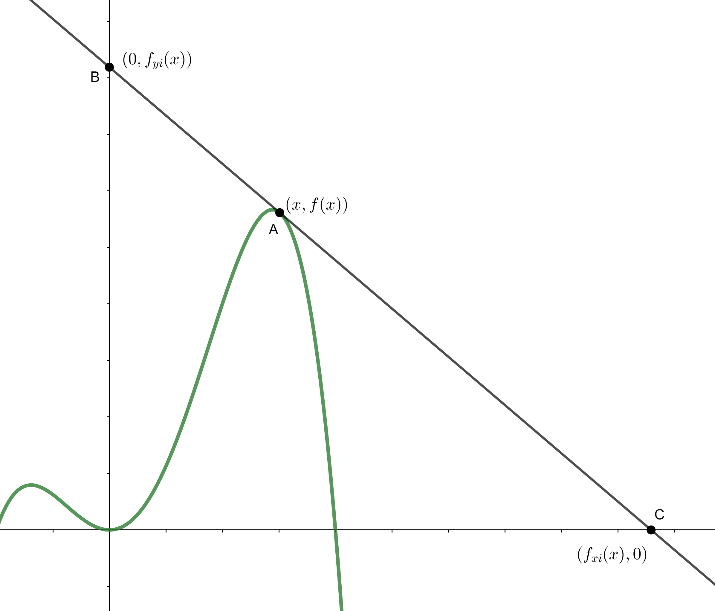
y-Intercept Formula. For a function f(x), the y-intercept formula is \(f_{yi}(x)=f(x)-x\cdot f'(x)\), where fyi(x) gives the y value of the point where a tangent to the curve at (x, f(x)) crosses the y-axis or (0, fyi(p)).
x-Intercept Formula. For a function f(x), the x-intercept formula is \(f_{xi}(x)= -\frac{f_{yi}(x)}{f'(x)} = x-\frac{f(x)}{f'(x)}\), where fxi(x) gives the y value of the point where a tangent to the curve at (x, f(x)) crosses the x-axis or (fxi(p), 0).
The image below show the representation of the designations.
Newton’s Method
When we search for the zeros of a polynomial function, we are looking for the point where the function crosses the x-axis. We can use the x-intercept formula for approximating zeros of a polynomial equation to any degree of accuracy. We can also use it for other functions, such as transcendental functions; however, that would require more than a paper and pencil. The x-intercept formula can also be written as \(\frac{x\cdot f'(x)-f(x)}{f'(x)}\). Using an initial value for x, we can approximate a zero r1 which may be close to x. This initial value for x will give the x-intercept of the tangent at x. But using the value obtained we can find the x-intercept again of the tangent and be closer to the zero. Repeating this procedure will bring the x-intercept closer and closer to the zero. Let’s use an example to illustrate the method using the function \(x^2-4=0\). We already know the zeros to be 2 and –2.
Let \(r_1 \approx x-\frac{f(x)}{f'(x)}=\) \(x-\frac{x^2-4}{2x}=\) \(\frac{x^2+4}{2x}\). We know one of the roots is 2 so we’ll choose an initial x value close to 2. Let’s say we choose a 6. Then, \({r}_{1}\approx \frac{6^2+4}{2(6)}=\frac{10}{3}\). Now, we iterate the process:
\(r_2 \approx \frac{(10/3)^2+4}{2(10/3)}=\frac{34}{15}\), \(r_3 \approx \frac{(34/15)^2+4}{2(34/15}=\frac{514}{255}\), \(r_4 \approx \frac{(514/255)^2+4}{2(514/255)}=\frac{131074}{65535}\approx \text{2}\text{.00006}\)We can see a pattern emerge: \(r_n = \frac{2\cdot 2^{2^n}+4}{2^{2^n}}\). The limit of this expression is 2. Sometimes, the values jump around instead of converging. In this case, you have to choose some other starting value.
Implicit Functions
The intercept formulas can also be used for implicit functions. Because we can find the slope through implicit differentiation, we can also find the x- and y-intercepts implicitly. Since the formula will not be a function, we’ll denote the x- and y-intercept formula for implicitly differentiated equations as follows.
If a function is defined implicitly, then its y-intercept formula, denoted as yyi, is given by \(y_{yi} = y-x\frac{dy}{dx}\) and its x-intercept formula, denoted as yxi, is given by \(y_{xi} = x-y\frac{dx}{dy}\).
The conic sections are great examples of implicit relationships. Here are examples for the three conics which are expressed as implicit equations.
Circles
The equation for circle is x² + y² = r² for radius of length r. Through implicit differentiation, the derivative is \(\frac{dy}{dx}=-\frac{x}{y}\). So the y-intercept formula is \(y_{yi} = y-x\left( \frac{-x}{y} \right)=\frac{x^2+y^2}{y}=\frac{r^2}{y}\), and x-intercept formula is \(y_{xi}=x-y\left( -\frac{y}{x} \right)=\frac{x^2+y^2}{x}=\frac{r^2}{x}\).
Ellipses
The equation for an ellipse is \(\frac{x^2}{a^2}+\frac{y^2}{b^2}=1\). The derivative is \(\frac{dy}{dx}=-\frac{b^{2}x}{a^{2}y}\). The y-intercept formula is \(y_{yi} = y+\frac{b^2 x^2}{a^{2} y} = \frac{a^2 y^2 + b^2 x^2}{a^2 y} = \frac{a^2 b^2}{a^2 y} = \frac{b^2}{y}\), and the x-intercpet formula is \(y_{xi} = \frac{a^2}{x}\).
Summary of Conics
The table below summarizes the slope, y-intercept, and x-intercept formulas.
| Conic | Equation | \(\frac{dy}{dx}\) | yyi | yxi |
| Circle | \(x^2+y^2=r^2\) | \(-\frac{x}{y}\) | \(\frac{r^2}{y}\) | \(\frac{r^2}{x}\) |
| Parabola | \(y = ax^2\) | \(2ax\) | \(-ax^2\) | \(x/2\) |
| Ellipse | \(\frac{x^2}{a^2}+\frac{y^2}{b^2}=1\) | \(-\frac{b^2 x}{a^2 y}\) | \(\frac{b^2}{y}\) | \(\frac{a^2}{x}\) |
| Hyperbola | \(\frac{x^2}{a^2}-\frac{y^2}{b^2}=1\) | \(\frac{b^2 x}{a^2 y}\) | \(-\frac{b^2}{y}\) | \(\frac{a^2}{x}\) |
| Hyperbola | \(-\frac{x^2}{a^2}+\frac{y^2}{b^2}=1\) | \(\frac{b^2 x}{a^2 y}\) | \(\frac{b^2}{y}\) | \(-\frac{a^2}{x}\) |
Differential Formulas
We can find an expression for the y-intercept and x-intercept for a given function or relation. However, what if we wanted to do the reverse? For example, is there a function f(x) such that a tangent at (x, f(x)) passes through the x-intercept at (x – 1, 0)? Or is there a function f(x) such that a tangent at (x, f(x)) passes through the y-intercept at (0, ln x)? Techniques for solving differential equations can help us find the general formulas such that a tangent at (x, f(x)) passes though (P(x), 0) or (0, Q(x)).
The General Solution to the X-Intercept Differential Equation
The x-intercept formula is given by \(y_{xi} = x-y\frac{dx}{dy}\). We let yxi = P(x) and solve for y in the x-intercept differential equation: \(x-y\frac{dx}{dy}=P(x)\). We wish to find a function y for which its x-intercept is given by P(x).
(i) \(x-y\frac{dx}{dy}=P(x)\)
(ii) \(\frac{x}{dx}-\frac{y}{dy}=\frac{P(x)}{dx}\) (Separate variables by dividing by dx.)
(iii) \(\frac{x-P(x)}{dx}=\frac{y}{dy}\)
(iv) \(\frac{dy}{y}=\frac{dx}{x-P(x)}\)
(v) \(\int \frac{dy}{y} = \int \frac{dx}{x-P(x)}\) (Integrate both sides.)
(vi) \(\ln \left| y \right| = \int \frac{dx}{x-P(x)}+C_1\)
(vii) \(\left| y \right| = e^{\int \frac{dx}{x-P(x)} + C_1} = Ce^{\int \frac{dx}{x-P(x)}}\)
If there exists a function y such that its x-intercept is given by the function P(x), then y is given by: \(y = Ce^{\int \frac{dx}{x-P(x)}}\)
We disregard the absolute value bars since C can be positive or negative.
Example 1
Problem: Find a function f such that its tangent at (x, f(x)) passes through (x², 0).
Solution: Using the formula, we must be able to integrate \(\int \frac{dx}{x-x^2}\) since P(x) = x². By means of partial fractions we have:
(i) \(\int \frac{dx}{x-x^2} = \int \frac{dx}{x(1-x)} = \) \(\int \frac{1}{x}+\frac{1}{1-x} \text{ } dx=\) \(\ln x - \ln (1-x) =\ln \frac{x}{1-x}\)
Therefore, the function \(y=Ce^{\ln [{x}/{(1-x)}]} = \frac{Cx}{1-x}\) whose tangent at some point p has its x-intercept at (p², 0).
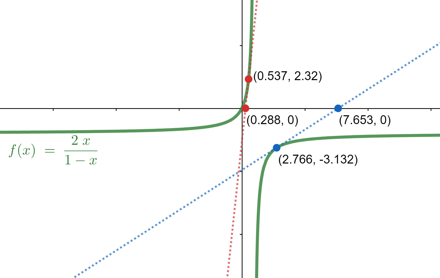
For the example above, we have graphed the function \(y = \frac{2x}{1-x}\), undoubtedly a hyperbola. Two tangents are shown in the two branches of the hyperbola. They both cross the x-axis at a point that is squared of the x value of the tangency. (Values are approximated.)
The General Solution to the Y-Intercept Differential Equation
For the general y-intercept formula, we must solve the y-intercept differential equation \(y-x\frac{dy}{dx} = Q(x)\), where yyi = Q(x). The solution to a first-order linear differential equation \(\frac{dy}{dx}+P_1(x)y = Q_1(x)\) is given by: \(ye^{\int P_1(x)dx} = \int Q_1(x)e^{\int P_1(x)dx}dx+C\). The y-intercept differential equation can be manipulated to fit the first-order linear differential equation form.
(i) \(y-x\frac{dy}{dx}=Q(x) \Rightarrow \frac{dy}{dx}-\frac{1}{x}y=-\frac{Q(x)}{x}\)
Thus, we have \(P_1(x)= -\frac{1}{x}\) and \(Q_1(x) = -\frac{Q(x)}{x}\). Substitution in the solution formula for the first-order linear differential equation gives us:
(iii) \(ye^{-\int 1/x \text{ }dx} = -\int \frac{Q(x)}{x}e^{-\int 1/x\text{ }dx}\text{ }dx + C\)
(iv) \(ye^{-\ln \left| x \right|} = -\int \text{ }\frac{Q(x)}{x}e^{-\ln \left| x \right|}\text{ }dx + C\)
(v) \(y = -x\int \frac{Q(x)}{x^2} \text{ }dx + Cx\)
We wish to make the formula less complicated, so we disregard the absolute value bars.
The function y such that its y-intercept is given by the function Q(x), then y is given by: \(y=Cx-x\int{\text{ }\frac{Q(x)}{{{x}^{2}}}dx}\). This function is graphed below showing two points of tangency and their x-intercepts.
Example 2
Problem: Find a function f(x) such that a tangent at (x, f(x)) passes through (0, ln x).
Solution: In this case Q(x) = ln x. Performing integration by parts, we have:
(i) \(y = Cx-x\int x^{-2}\ln x \text{ } dx=\) \(Cx-x\left[ -x^{-1}\ln x+\int x^{-2} \text{ }dx \right] =\) \(-x\left( -\frac{\ln x}{x}-\frac{1}{x} \right) = Cx+1+\ln x\)
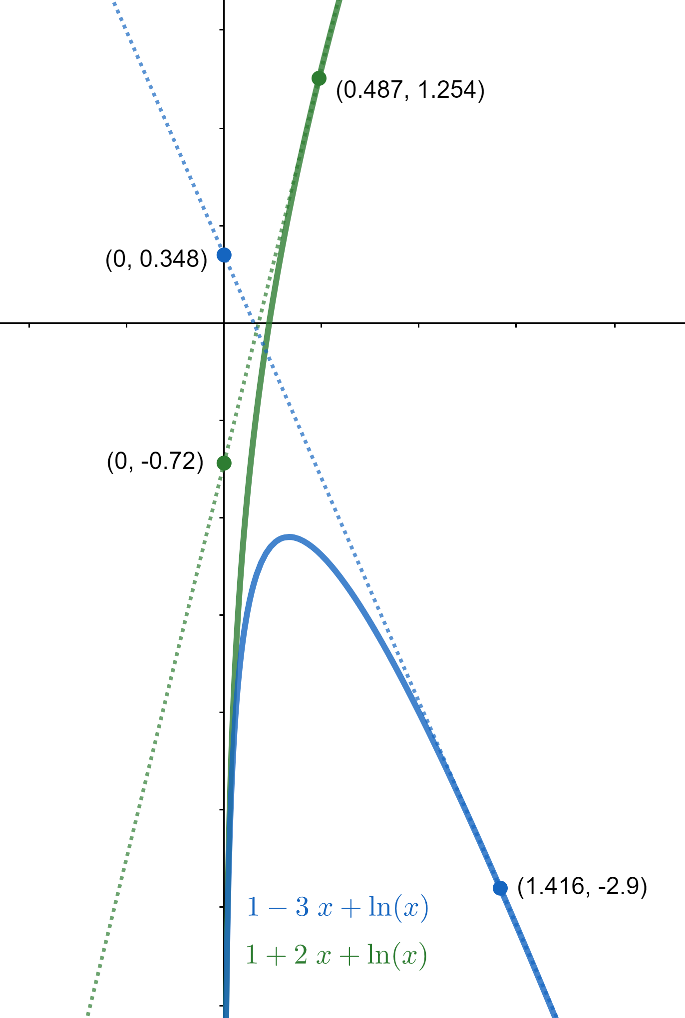
The general solution is \(Cx+1+\ln x\), for all real C. This function is graphed on the right. The green function is when C = 2: \(f(x) = 1+2x+\ln(x)\). The blue function is when C = –3: \(f(x) = 1 - 3x + \ln(x)\). The y-intercept is independent of C and the tangent always crosses the y-axis at ln(x).
If you were to track the tangent points on this graph and place them at x = 1, then the y-intercepts will be 0 because ln(1) = 0. Because C = –3 in the blue graph, it has a relative mamixum, which can be found at x = 1/3. At this point, since the tangent is horizontal, it follows that f(1/3) = fyi(1/3) ≈ –1.098.
If C is positive, the derivative has no zeroes. Hence, there are no relative extrema.
In the above intercept differential equations, the x-intercept and y-intercept were functions of x. However, the intercepts do not have to be functions. If the x-intercept differential equation is y dependent, then the equation would be \(x-y\frac{dx}{dy}=P(y)\), where P is a relation of y. In this equation, we cannot directly solve for y, but we can solve for x. We can manipulate this differential equation into the form \(\frac{dx}{dy}-\frac{1}{y}x=-\frac{P(y)}{y}\). Using the solution to the first-order linear differential equation, we can solve for x to be \(x = Cy-y\int \frac{P(y)}{y^2}dy\).
If the x-intercept of a curve is given by P(y) and y dependent, then the curve is defined by the equation \(x = Cy-y\int \frac{P(y)}{y^2}dy\). The curve is a function only if we can isolate y.
Constant Ratio Curves
An interesting excursion with the intercept formulas are the constant ratio curves given by the equation \(y=\frac{C}{x^{\frac{1}{k}}}\). Depicted below is the curve for k = 4 and C = 1.
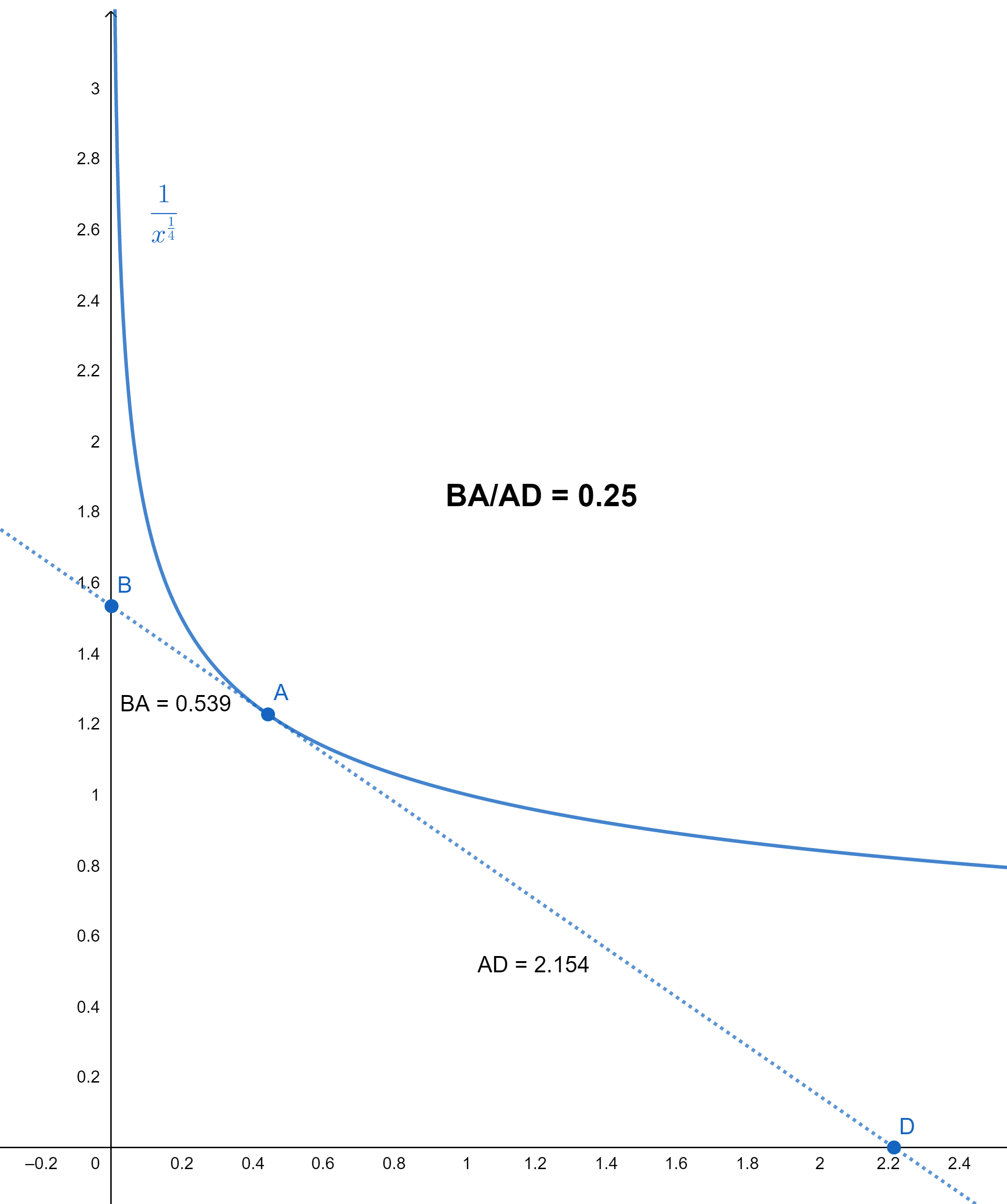
In this family of curves, the ratio AB to AD is always constant for a point B that is tangent to the curve at A. This ratio is equal to 1/k. The constant C plays no role in the ratio. Therefore, for all C, the curve \(y=\frac{C}{x^{\frac{1}{5}}}\) will produce a ration of 1/5.
When k = 1, we have a family of hyperbolas. The tangents of the hyperbola divides the segment into equal parts.
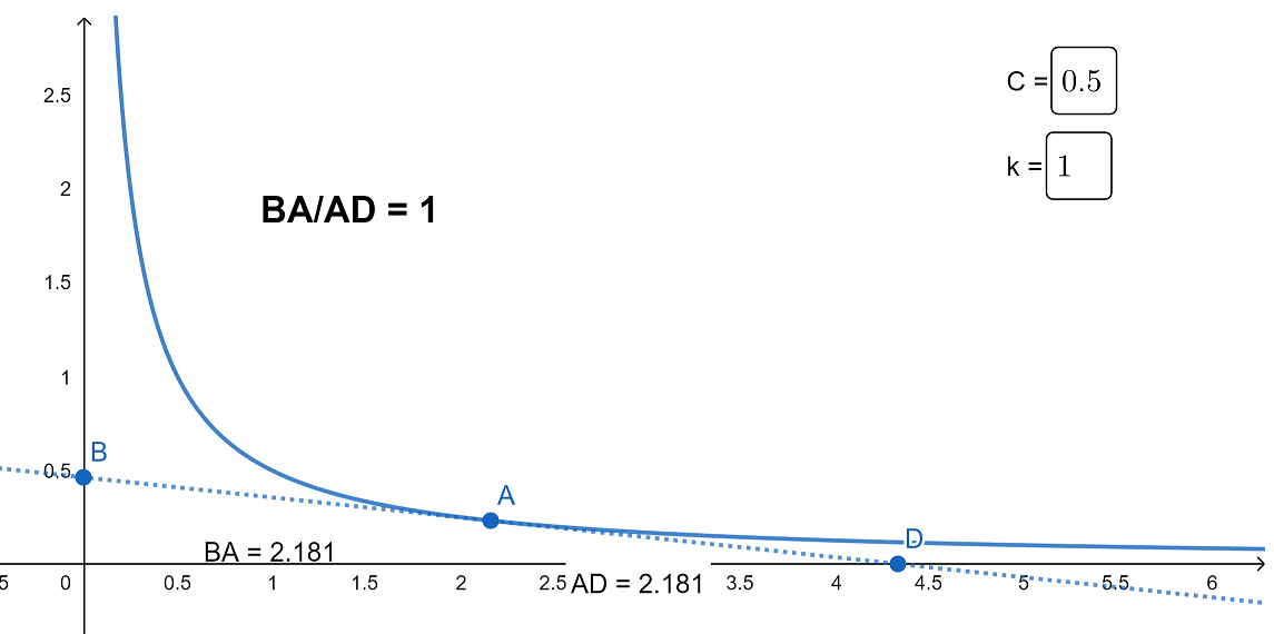
Above image shows the equation \(y=\frac{0.5}{x^2}\) graphed. It shows that the tangent is divided into two at the point of tangency.
Even if k is less than 1, the constant ratio holds true. As a matter of fact, when the ratio is less than 0, the equation becomes a simple polynomial. If the ratio is –1/2, the equation is \(y = \frac{1}{2}x^2\) which is the familiar parabola. In this case where the point of tangency is not in the middle of the x- and y-intercepts, the ratio we measure is from the point of tangency to the y-axis with the point of tangency to the x-axis. The segment itself is dissected into half by the axis, as can be seen below.

Example 3
In general, a tangent to the simple polynomial \(y = x^n\) is divided in a ratio of 1 to (n – 1) by the x-intercept. Let’s prove this. Let point P be given by (p, pn) on the curve. The slope of the tangent at this point is:
(i) \(y'(p) = np^{n-1}\)
The y-intercpet is given by:
(ii) \(y_{yi}(p) = p^n - p(np^{n-1}) = (1-n)p^n\).
So the y-intercept is located at \((0, (1-n)p^n)\). The x-intercept is given by:
(iii) \(y_{xi}(p) = p - p^n\cdot\frac{1}{np^{n-1}} = p-\frac{1}{n}p = \frac{n-1}{n}p\).
So the x-intercept is located at \(\left(\frac{n-1}{n}p, 0\right)\). Now, we find the distances between the tangent point with the intercept points. First, the distance, dy, between the tangent point (p, pn) and y-intercept \((0, (1-n)p^n)\):
(iv) \(d_y = \sqrt{(p - 0)^2 + [p^n - (1-n)p^n]^2}\)
(v) \(d_y = \sqrt{p^2 + n^2p^{2n}}\)
(vi) \(d_y = p\sqrt{1 + n^2p^{2n-1}}\)
Now, we will find the distance between the tangent point (p, pn) and x-intercept \(\left(\frac{n-1}{n}p, 0\right)\):
(vii) \(d_x = \sqrt{\left(p - \frac{n-1}{n}p\right)^2 + (p^n - 0)^2}\)
(viii) \(d_x = \sqrt{\left(\frac{p}{n}\right)^2 + p^{2n}}\)
(xv) \(d_x = \frac{p}{n}\sqrt{1 + n^2p^{2n-2}}\)
When we take the ratio of the distances, we get \(\frac{d_y}{d_x} = \frac{p\sqrt{1 + n^2p^{2n-1}}}{\frac{p}{n}\sqrt{1 + n^2p^{2n-2}}} = n\). This is exactly what we expected. The ratio between the distances is n. And because the point of tangency is not between the intercepts, the segment from the point of tangency to the y-intercept is divided in a ratio of 1 : (n – 1) by the x-intercept.
Last Word
A great application of the x- and y-intercept formulas is characterizing the tangent-generated curve. You can read about this topic here: tangent-generated curve.